
Geotechnical engineering libraryContact
 benesch
Railroad Geotechnical Services Manual | Primary Source: USACE EM 1110-1-1804 All equations and parameters expressed in English (Imperial) units throughout.
Apps on dirtbert.com that support this chapter. Each one runs in a web browser on a desktop or a phone, with nothing to install. How to use the apps (I.3). Tools marked TOOLS open in the Geotechnical Analysis Suite (Benesch sign-in); the orange card below lists each one by section.
NANCY pages ask you to accept the Use and Disclaimers once in each browser.
Calculators and workbook tools from the Benesch Geotechnical Analysis Suite that support this chapter: 11 interactive calculators and 2 workbook guides. Each one is also placed inside the section it supports, in an orange tools strip.
| SF | Bearing Capacity — AASHTO LRFDUsed in 11.2 Shallow Foundation Bearing Capacity — Vesić General Equation | Calculator ▸ | Guide |
| SF | Bearing Capacity — Terzaghi & VesićUsed in 11.2 Shallow Foundation Bearing Capacity — Vesić General Equation | Calculator ▸ | Guide |
| SF | Footing on SlopeUsed in 11.2 Shallow Foundation Bearing Capacity — Vesić General Equation | Calculator ▸ | Guide |
| SF | Rock — Shallow FoundationsUsed in 11.2 Shallow Foundation Bearing Capacity — Vesić General Equation | Calculator ▸ | Guide |
| SF | Machine Foundation Design & Dynamic Soil PropertiesUsed in 11.2 Shallow Foundation Bearing Capacity — Vesić General Equation | Calculator ▸ | Guide |
| DF | Drilled Shaft Design — Soils, LRFD (AASHTO 2018)Used in 11.5 Deep Foundation Bearing Capacity | Calculator ▸ | Guide |
| DF | Rock-Socket Drilled Shaft DesignUsed in 11.5 Deep Foundation Bearing Capacity | Calculator ▸ | Guide |
| DF | Pipe Pile API AnalysisUsed in 11.5 Deep Foundation Bearing Capacity | Calculator ▸ | Guide |
| DF | Pile Length — LRFD Modified IDOT/ENR FormulaUsed in 11.5 Deep Foundation Bearing Capacity | Calculator ▸ | Guide |
| DF | Pile Driving with DowndragUsed in 11.5 Deep Foundation Bearing Capacity | Calculator ▸ | Guide |
| DF | LPILE Lateral p-y MultiplierpreliminaryUsed in 11.6 Pile Group Efficiency | Calculator ▸ | Guide |
| DF | Auger Cast Pile Design — ASD (GEC 8)Used in 11.5 Deep Foundation Bearing Capacity | guide only | Guide |
| DF | Broms Method — Lateral PileUsed in 11.6 Pile Group Efficiency | guide only | Guide |
Tools open on dirtbert.com and need the Benesch sign-in. Drafts pending Benesch final review, not for use in design.
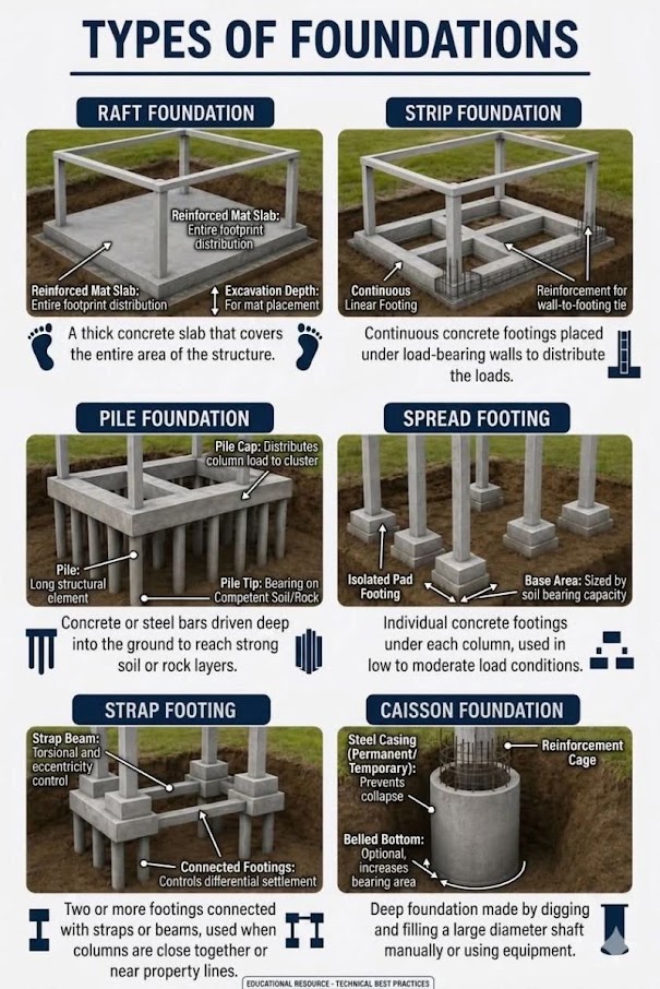
General topic illustrations from Benesch's shared geotechnical graphics library, related to this chapter's subject matter — not the numbered figures called out in the text above. Click any image to view it full size.
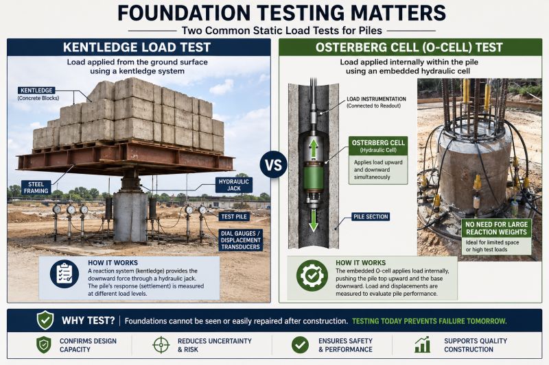
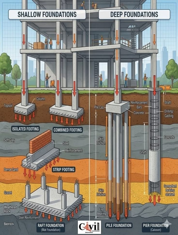
Foundation bearing capacity governs the structural adequacy of every load-transfer element in railroad infrastructure — bridge abutments and piers, signal equipment foundations, grade crossing slabs, retaining wall footings, building slabs at intermodal yards, and pile-supported overhead structures. This chapter develops the complete bearing capacity framework for shallow and deep foundations under railroad loading, applying the Vesić generalized bearing capacity equation to strip, rectangular, and circular footings; eccentric and inclined loading from longitudinal braking and lateral wind; and pile capacity by the α-method (cohesive soils), β-method (cohesionless soils), and Meyerhof SPT-based method. Cooper E-80 live loads with client-specific dynamic amplification factors are translated into equivalent static foundation pressures. Worked examples address a spread footing under an NSRR bridge abutment, a drilled shaft at a BNSF bridge pier, and a pile group at a UPRR intermodal crane rail. All nine railroad clients impose unique requirements for minimum factors of safety, pile type preferences, and structural review coordination; these are integrated throughout. Cross-references are provided to Chapter 12 (Settlement Analysis), Chapter 13 (Slope Stability), Chapter 14 (Seismic/Liquefaction), and Chapter 2 (Railroad Track Subgrade).
The correlations below are used or referenced in this chapter. Each is a statistical fit to a particular data set, so a value from one is an estimate: it applies only within the materials and ranges stated, carries the scatter of the original data, and must be confirmed by site-specific testing or calibration before it is relied on for design.
When an equation is used, note it with the result: give the equation ID and source, state that the soil or rock is within its range of applicability, mark the value as correlated (not tested), and record the limitation that governs. The Empirical Equations & Correlations reference has every entry with its full references.
Variables. Nm = field blow count; ERm = measured hammer energy ratio (%); CB = borehole diameter (1.0 for 65–115 mm, 1.05 for 150 mm, 1.15 for 200 mm); CS = sampler (1.0 standard, 1.1–1.3 liner-less); CR = rod length (0.75 <3 m; 0.8 3–4 m; 0.85 4–6 m; 0.95 6–10 m; 1.0 >10 m)
Use. All soils tested by SPT (ASTM D1586). Normalizes blow count to 60% of theoretical free-fall energy, the basis for most U.S. correlations.
Limitations. CE ranges ~0.5–1.6 depending on hammer type; use measured energy (ASTM D4633) where available. Rod-length factor ranges differ between Skempton (1986) and Youd et al. (2001).
Source. Skempton 1986; Youd et al. 2001 · In this chapter: 11.11, 11.13 · Full entry and references
Variables. φ' = peak drained triaxial friction angle
Use. Clean, uncemented quartz sands. Curve fit to Schmertmann's (1975) chart.
Limitations. Underpredicts in gravels, overpredicts in silty/micaceous sands. Do not use in clays or cemented soils.
Source. Kulhawy & Mayne 1990 (after Schmertmann 1975) · Full entry and references
Variables. (N1)60 from IS-02
Use. Granular soils; regression of the Peck, Hanson & Thornburn (1974) chart. Common in U.S. DOT practice.
Limitations. Conservative for dense sands. Not valid beyond chart range (~N > 50).
Source. Wolff 1989 (fit to Peck et al. 1974) · Full entry and references
Variables. N1 = N normalized to 98 kPa, Japanese energy (~78% ER in original study)
Use. Based on high-quality (frozen) undisturbed samples of Holocene and Pleistocene sands; N1 ≈ 3–40.
Limitations. Convert energy basis before using U.S. N60. Scatter about ±3°.
Source. Hatanaka & Uchida 1996 · Full entry and references
Variables. f1 varies with plasticity index
Use. Insensitive, overconsolidated clays and weak rocks (U.K. data); PI ≈ 15–65%.
Limitations. Very large scatter; not reliable in soft or sensitive clays where N is very low. Use CPT, vane, or lab tests for design Su.
Source. Stroud 1974 · Full entry and references
Variables. Nkt = empirical cone factor, typically 10–20 (average ≈ 14); decreases with increasing Bq
Use. Fine-grained soils penetrated undrained (Ic > ~2.6).
Limitations. Nkt depends on reference test (vane, CIUC, DSS) and plasticity; calibrate locally. Use Nkt toward upper end for conservative Su.
Source. Lunne et al. 1997 · Full entry and references
Variables. Bracketed term = Qt1 (normalized tip resistance)
Use. Clean, unaged, uncemented quartz sands; based on calibration chamber data.
Limitations. Overpredicts in compressible (carbonate, micaceous) sands; underpredicts in aged/cemented sands.
Source. Kulhawy & Mayne 1990 · Full entry and references
Variables. σci = intact UCS; mi = intact rock constant; D = disturbance factor (0 undisturbed – 1 heavily blasted)
Use. Isotropic, heavily jointed rock masses (4+ joint sets) or intact rock.
Limitations. Not for rock masses where failure is controlled by one or two discrete discontinuity sets; use structural (kinematic) analysis there. D strongly affects results in slopes.
Source. Hoek et al. 2002 · Full entry and references
Foundations for railroad structures must support not only static dead loads but also highly dynamic live loads, impact, braking, and lateral forces that are unique to rail operations. Cooper E-80 loading — 80 kips per axle for the locomotive and 80 kips per axle for the tender — remains the standard design live load for Class I structures per AREMA MRE Chapter 8. Dynamic load factors (DLF) applied to axle loads before distribution to foundation elements range from 1.20 for slow-speed industrial trackage (G&W Engineering Bulletins, EB-2021) to 1.50 for high-speed Amtrak NEC operations (Amtrak Engineering Standards, ES-B-2023).
Each railroad client imposes specific foundation design requirements beyond AREMA MRE minima:
Our role as consultants is to deliver foundation designs that satisfy both structural adequacy (FS against failure) and serviceability (settlement limits per Chapter 12), calibrated to each client's operational environment and proprietary standards.
Reference graphics
Reference graphics · click to zoom
Selig and Waters compare two ways to model the track as a footing:
The strip-footing case gives a much lower capacity and governs. Capacity rises with granular depth H.
Slope-stability approach. A method-of-slices analysis is a conservative, two-dimensional check. The book applies a design load of 4,880 psf over the 8.5-ft tie length. A loaded 100-ton car is equivalent to about 1,400 psf, roughly 30% of that design load. An analysis FS of 1.0 therefore means the car is at about 30% of the failure load. The book treats that as the upper limit for avoiding large plastic deformation under repeated loading. At an analysis FS of about 0.3, expect massive failure.
| Subgrade strength | Analysis FS (target ≥ 1.0) |
|---|---|
| c = 0, φ = 30° | ≈ 1.1 |
| c = 1,000 psf, φ = 0 | ≈ 1.1 |
| c = 1,500 psf | 1.6 |
| c = 2,000 psf | 2.1 |
| c = 3,000 psf | 3.0 |
FS is roughly linear in c and in φ. A cut section gives about the same FS as flat ground. Embankments give lower values, with up to about a 30% reduction at a 1:1 (45°) side slope with a narrow shoulder. On an embankment the critical surface is deeper.
After Selig & Waters (1994), ch. 10. Full reference under Supplemental Sources.
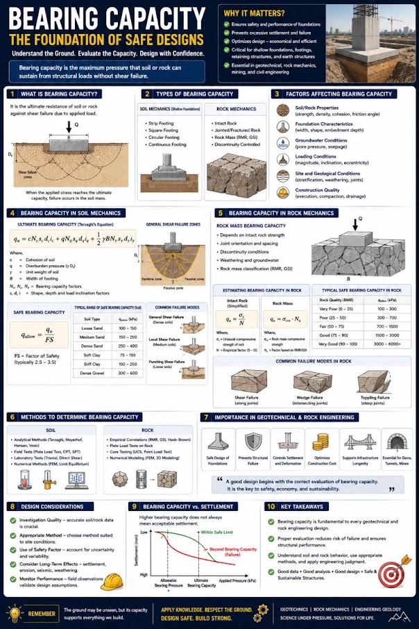
The Vesić (1973) generalization of Terzaghi's original equation is the standard for computing ultimate unit bearing capacity q_ult for shallow foundations:
Reference graphics
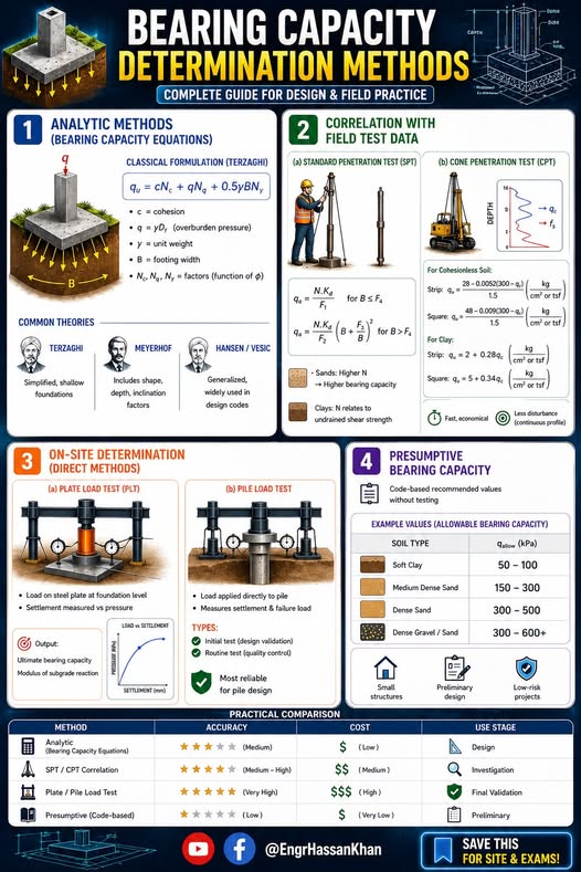
q_ult = c · Nc · Fcs · Fcd · Fci
+ q · Nq · Fqs · Fqd · Fqi
+ 0.5 · γ · B · Nγ · Fγs · Fγd · Fγi
Where:
Nq = e^(π·tan φ') · tan²(45 + φ'/2)
Nc = (Nq − 1) · cot φ' (use Nc = 5.14 when φ' = 0)
Nγ = 2(Nq + 1) · tan φ'
| φ' (°) | N_c | N_q | N_γ | Typical Soil Description |
|---|---|---|---|---|
| 0 | 5.14 | 1.00 | 0.00 | Soft–medium clay (UU condition) |
| 5 | 6.49 | 1.57 | 0.45 | Soft clay with minor sand |
| 10 | 8.35 | 2.47 | 1.22 | Silty clay |
| 15 | 10.98 | 3.94 | 2.65 | Stiff clayey silt |
| 20 | 14.83 | 6.40 | 5.39 | Dense silt, loose sand |
| 25 | 20.72 | 10.66 | 10.88 | Medium-dense sand |
| 30 | 30.14 | 18.40 | 22.40 | Dense sand, gravel-sand |
| 35 | 46.12 | 33.30 | 48.03 | Dense gravel |
| 40 | 75.31 | 64.20 | 109.4 | Very dense gravel |
| 45 | 133.9 | 134.9 | 271.8 | Dense rock fill |
For a rectangular footing of width B and length L (L ≥ B):
Fcs = 1 + (B/L)(Nq/Nc)
Fqs = 1 + (B/L) tan φ'
Fγs = 1 − 0.4(B/L)
For a strip footing: B/L → 0, so F_cs = F_qs = F_γs = 1.0. For a circular footing (B = L): B/L = 1.0.
No additional content.
Fcd = 1 + 0.4(Df/B)
Fqd = 1 + 2·tan φ'·(1 − sin φ')²·(Df/B)
Fγd = 1.0
For D_f/B > 1, replace D_f/B with arctan(D_f/B) in radians in the F_qd expression.
For a resultant load inclined at angle β from vertical (due to braking or wind forces):
Fci = Fqi = (1 − β/90)²
Fγi = (1 − β/φ')²
β is in degrees. For purely vertical loading, β = 0 and all inclination factors = 1.0.
No additional content.
Reference graphics
Reference graphics · click to zoom
q_allow = (q_ult − q) / FS + q
Where q = surcharge at footing base; FS = factor of safety (typically 3.0 for railroad structures with limited investigation; 2.5 with comprehensive investigation per G&W EB).
The net allowable bearing pressure is:
q_net,allow = (q_ult − q) / FS
For railroad bridge abutments, CSXT ES and NSR ESM require FS ≥ 3.0. For yard and siding structures, G&W EB permits FS = 2.5 with borings at every foundation location.
Strong layer over weak layer. A compacted ballast/subballast section or desiccated crust over soft clay is the typical railroad profile, and the Vesić equation (which assumes one homogeneous soil) overestimates capacity there. Das presents the Meyerhof and Hanna (1978) method: when the strong layer thickness H is small relative to B, the footing punches through the top layer (resisted by adhesion and passive force on vertical planes below the footing edges) and then fails the lower layer in general shear:
qu = qb + 2(Ca + Pp sin δ′)/B − γ1H ≤ qt (capacity of the top layer alone)
where qb is the bearing capacity of the weaker layer and Ca = c′aH is the adhesion force. If H is large, the failure surface stays in the top layer and qt governs. For signal and equipment foundations on a thin working platform over soft subgrade, check this mechanism.
Footing at the top of a slope. Signal masts, catenary poles and bridge abutments often sit on or near an embankment crest. Meyerhof (1957) gives qu = c′Ncq + ½γBNγq, with Ncq and Nγq charted against slope angle, footing setback b/B, embedment Df/B and, for clay, the stability number Ns = γH/cu. Capacity increases with setback distance (Das charts b/B from 0 to about 6); a footing right at the crest can have a small fraction of its level-ground capacity. Always follow with a global slope stability check (Chapter 13).
Source: Das, B. M. Principles of Foundation Engineering. Cengage Learning
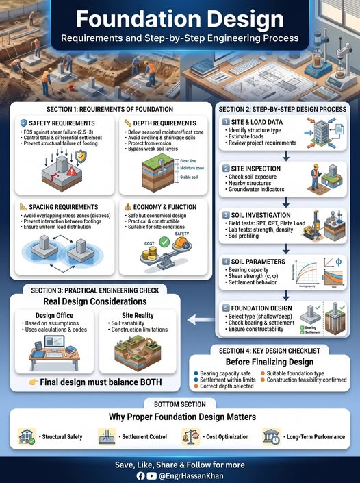
For signal houses, small culvert headwalls and other minor railroad structures — or to sanity-check a Vesić result — NAVFAC DM-7.02 (Table 1) gives presumptive allowable pressures intended to provide adequate safety against failure and avoid detrimental settlement of individual footings:
Table 11-S1. Presumptive allowable bearing pressure, tsf (NAVFAC DM-7.02, Table 1, abridged)
| Bearing material | Consistency | Range | Recommended |
|---|---|---|---|
| Massive crystalline igneous/metamorphic rock (granite, basalt, gneiss) | Hard, sound | 60–100 | 80 |
| Foliated metamorphic rock (slate, schist) | Medium hard, sound | 30–40 | 35 |
| Hard cemented shale, siltstone, sandstone, limestone without cavities | Medium hard, sound | 15–25 | 20 |
| Weathered or broken bedrock (RQD < 25), except argillaceous | Soft rock | 8–12 | 10 |
| Compaction shale / argillaceous rock, sound | Soft rock | 8–12 | 10 |
| Glacial till, hardpan (GW-GC, GC, SC) | Very compact | 8–12 | 10 |
| Gravel, gravel–sand (GW, GP, SW, SP) | Very compact / medium / loose | 6–10 / 4–7 / 2–6 | 7 / 5 / 3 |
| Coarse to medium sand (SW, SP) | Very compact / medium / loose | 4–6 / 2–4 / 1–3 | 4 / 3 / 1.5 |
| Fine to medium sand, silty or clayey sand (SW, SM, SC) | Very compact / medium / loose | 3–5 / 2–4 / 1–2 | 3 / 2.5 / 1.5 |
| Inorganic clay (CL, CH) | Very stiff–hard / medium–stiff / soft | 3–6 / 1–3 / 0.5–1 | 4 / 2 / 0.5 |
| Inorganic silt, varved silt-clay-fine sand | Very stiff–hard / medium–stiff / soft | 2–4 / 1–3 / 0.5–1 | 3 / 1.5 / 0.5 |
NAVFAC’s notes matter for railroad use: controlled compacted fill takes the value of the equivalent natural soil; organic soil and uncompacted fill (common in old railroad embankments) must be investigated case by case; on compressible fine-grained soil, settlement generally governs; and a rock value may never exceed the intact UCS. Transient wind or earthquake loads may increase the pressure by up to one-third. Presumptive values are not a substitute for analysis where differential settlement matters, soils are soft, or groundwater is shallow.
Source: Naval Facilities Engineering Command (1986). Foundations and Earth Structures, Design Manual 7.02 (NAVFAC DM-7.02)
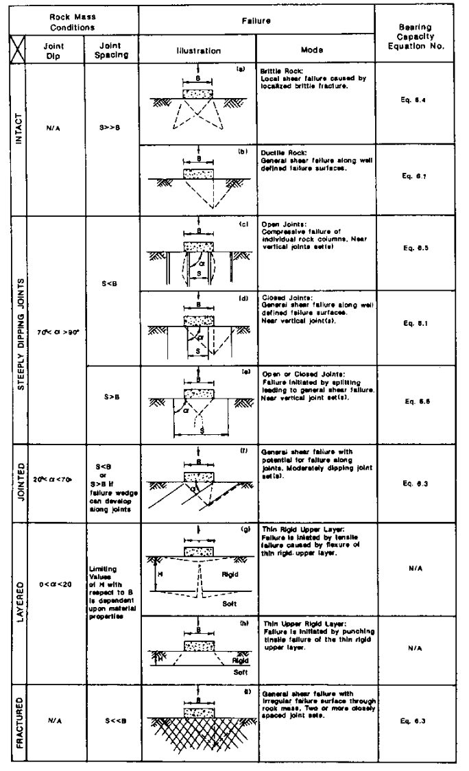
USACE EM 1110-1-2908 notes that rock foundation design is usually controlled by settlement, sliding or overturning, but bearing must still be checked, and the failure mode depends on joint spacing S relative to footing width B, joint orientation and condition (Figure 11-S1):
For non-strip footings EM 1110-1-2908 applies Sowers’ shape corrections: Nc × 1.2 (circular), 1.25 (square), 1.12 (L/B = 2), 1.05 (L/B = 5); Nγ × 0.70, 0.85, 0.90, 0.95 respectively. Because rock masses usually have a large margin, USACE recommends starting from lower-bound c and φ.
Source: U.S. Army Corps of Engineers (1994). Rock Foundations. EM 1110-1-2908
Railroad abutment footings routinely carry eccentric loads due to moment from earth pressure, live load surcharge, and longitudinal braking. The effective area method (Meyerhof 1953) reduces the footing dimensions to eliminate tension:
Reference graphics
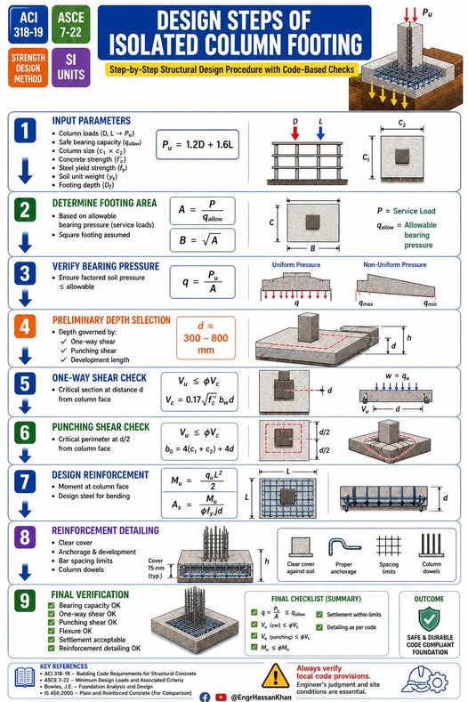
B' = B − 2·e_B
L' = L − 2·e_L
Where e_B = M_B / P and e_L = M_L / P are eccentricities (ft) computed from resultant moments about the footing centroid. AREMA MRE Chapter 8 requires that the resultant fall within the middle third of the footing (e ≤ B/6) for unfactored loading.
Bearing capacity calculations use B' and L' in all equations; settlement analysis (Chapter 12) uses the full B and L for stress distribution.
The Cooper E-80 equivalent uniform load is commonly taken as 4,000 psf on the rail seat area for bridge abutment backwall pressure analysis. For footing design, the geotechnical engineer converts the wheel load train to a resultant foundation reaction:
Reference graphics
P_design = (DL + LL·DLF) / A_footing
Where:
Typical Cooper E-80 bridge seat reactions for a 60-ft simple span are 320–380 kips per bearing. With DLF = 1.30 (BNSF EI main-line default), the dynamic-factored reaction is 416–494 kips per bearing.
The usual simplification treats the tie as a beam overhanging both rails, with a uniform ballast pressure over a length 2·ℓexc under each rail. Field measurements (ORE, 1973) show a different distribution: pressure concentrated under the rail seats, falling to about a quarter of the peak at the tie center (Figure 11-12). The peak pressure is given empirically by:
where P = axle load (2 × wheel load), α = tie width, L = tie length and ℓexc = distance from tie end to rail seat. For an E-80 or heavy-axle check of ballast and subballast bearing, this measured shape is a better basis for the pressure under the rail seat than a uniform average over the whole tie.
Figures · click to zoom
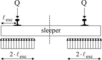
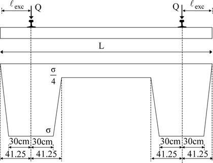
After Profillidis (2014), §11.8, Eq. 11.1, Figs. 11.10–11.11; after ORE D71 (1973). Full reference under Supplemental Sources.
Reference graphics
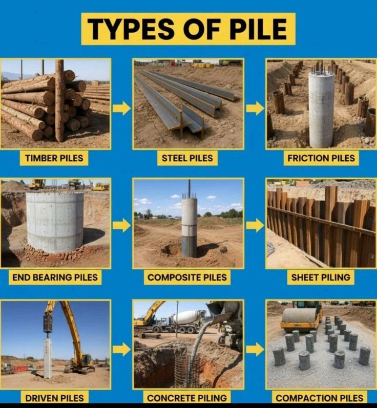
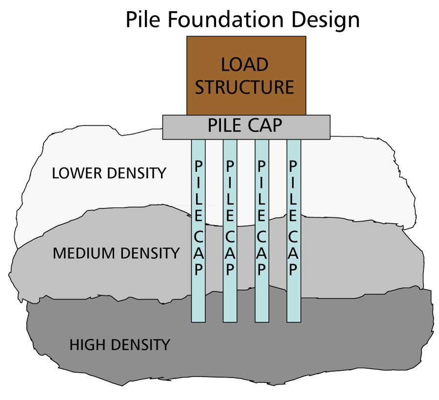
Reference graphics · click to zoom
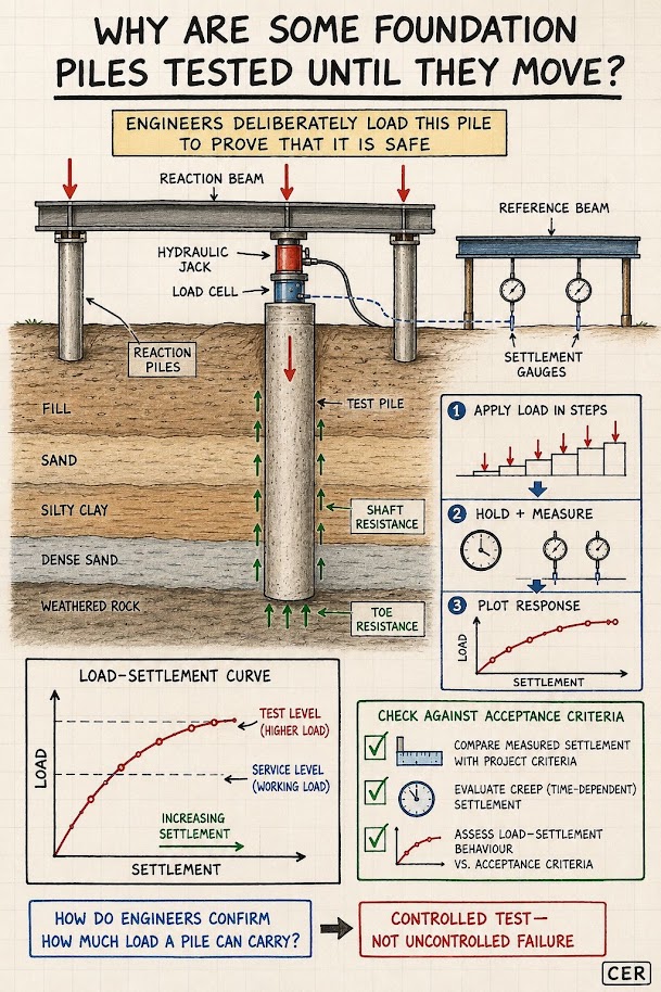
Total pile capacity Q_ult is the sum of side friction Q_s and tip resistance Q_p:
Reference graphics
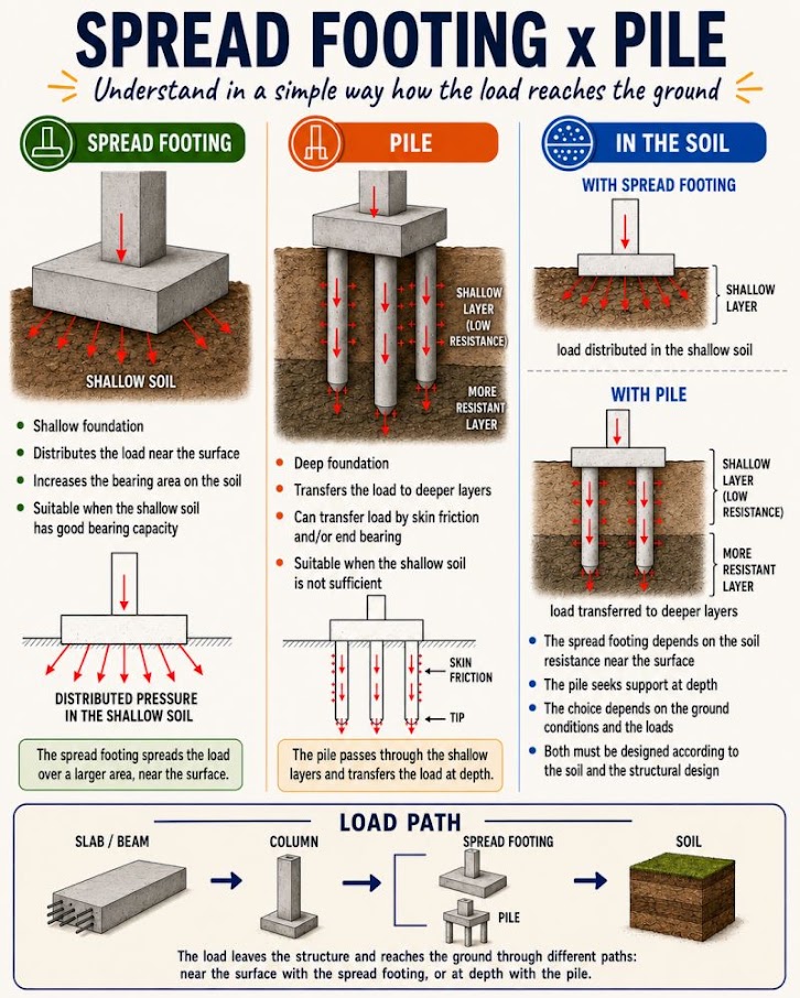
Q_ult = Q_s + Q_p = Σ(f_s · A_s) + q_p · A_tip
Where:
Allowable pile capacity:
Q_allow = Q_ult / FS
UPRR EIM specifies FS = 2.5 with static load test confirmation; FS = 3.0 without load testing. BNSF EI specifies FS = 2.5 with CAPWAP; FS = 3.5 without dynamic testing.
The α-method (API RP 2A) computes unit skin friction in cohesive soils as a fraction of undrained shear strength:
Reference graphics
f_s = α · su
α = 0.5 · ψ^(−0.5) when ψ ≤ 1.0
α = 0.5 · ψ^(−0.25) when ψ > 1.0
Where ψ = s_u / σ'_v (undrained strength ratio). For railroad bridge piles in typical alluvial clay (s_u = 800–1,200 psf; σ'_v = 1,500–2,500 psf), ψ ≈ 0.4–0.6 and α ≈ 0.65–0.79.
Unit tip resistance for closed-end pipe piles in clay:
q_p = 9 · su (at pile tip)
In cohesionless soils, skin friction is computed as a fraction of the effective overburden stress:
Reference graphics
f_s = β · σ'_v
β = K · tan(δ)
Where:
Typical β values: 0.25–0.40 for steel H-piles in medium-dense sand. UPRR EIM uses β = 0.30 as a default for HP14×117 piles in alluvial sand without site-specific testing.
Unit tip resistance in cohesionless soils (Meyerhof):
q_p = σ'_v · Nq* (limited to 1.0 ton/ft² × Nq* ≤ q_p,lim)
Nq* = bearing capacity factor for pile tip (Vesić table, typically 50–80 for dense sand, φ' = 35–40°). Limiting tip resistance for driven piles in sand is typically capped at 100–150 tsf per AREMA MRE Chapter 7.
For driven displacement piles, the Meyerhof (1976) empirical method using corrected SPT blow counts is widely used for preliminary designs and for G&W and regional railroad projects where detailed lab testing is not available:
Reference graphics
f_s = 0.02 · N60 (tsf)
q_p = 0.4 · N60 · (Db/B) ≤ 4·N60 (tsf)
Where:
For piles in clay, Meyerhof recommends:
f_s = su/500 (tsf)
q_p = 9·su/2000 (tsf)
Where s_u is in psf. These empirical correlations are suitable for preliminary design and contractor quantity estimates; CSXT ES and NSR ESM require verification by static or high-strain dynamic load testing.
Client-specific safety factors in Section 11.5.1 are consistent with FHWA practice, which links the factor of safety for driven piles to the field verification method:
Table 11-S2. Recommended FS by construction control method (FHWA NHI-05-042, Table 9-1)
| Construction control method | FS |
|---|---|
| Static load test (ASTM D1143) with wave equation analysis | 2.00 |
| Dynamic testing (ASTM D4945) with wave equation analysis | 2.25 |
| Indicator piles with wave equation analysis | 2.50 |
| Wave equation analysis only | 2.75 |
| Gates dynamic formula | 3.50 |
Only resistance from layers that give long-term support counts toward the design load: exclude shaft resistance in soil that can scour in the design flood and in soft compressible layers. Those layers still resist driving, so the driving resistance the hammer must overcome is larger than the design capacity — a frequent source of under-sized hammers at railroad stream crossings.
Table 11-S3. Soil setup factors (Rausche et al., 1996, in FHWA NHI-05-042, Table 9-20)
| Predominant soil along shaft | Range | Recommended |
|---|---|---|
| Clay | 1.2–5.5 | 2.0 |
| Silt–clay | 1.0–2.0 | 1.0 |
| Silt | 1.5–5.0 | 1.5 |
| Sand–clay | 1.0–6.0 | 1.5 |
| Sand–silt | 1.2–2.0 | 1.2 |
| Fine sand | 1.2–2.0 | 1.2 |
| Sand | 0.8–2.0 | 1.0 |
| Sand–gravel | 1.2–2.0 | 1.0 |
Setup factors should be confirmed with local experience and restrike testing. The opposite effect, relaxation, occurs in dense saturated fine sands and non-cohesive silts (dilation and temporary suction at the toe) and in some laminated shales (release of locked-in horizontal stress). Where relaxation is possible, capacity must be verified by restrike or load test after pore pressures equilibrate, not at end of driving.
Source: Hannigan, P. J., Goble, G. G., Likins, G. E. and Rausche, F. (2006). Design and Construction of Driven Pile Foundations, Vol. I. FHWA NHI-05-042
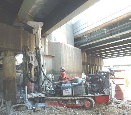
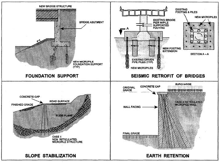
Where soft ground is too deep to remove economically, track load can be carried to competent soil on piles beneath a load-transfer platform. Micropiles are small-diameter drilled and grouted shafts. Screw piles are rotated in with a helix tip, need no excavation or grout, and can be installed from a rail-mounted rig, including in winter. At Lac la Biche Sub Mile 173.48, 68 piles of 18-in. diameter in two flights at 10° from vertical underpinned about 400 ft of track settling into peat.
Figures · click to zoom
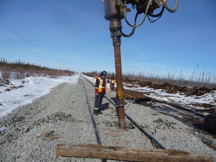
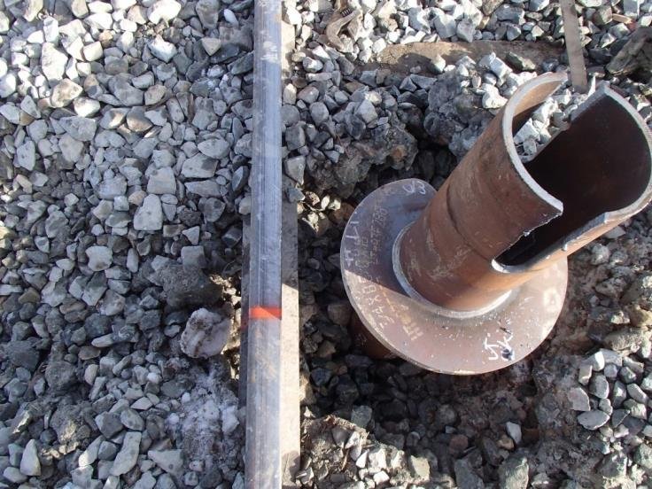
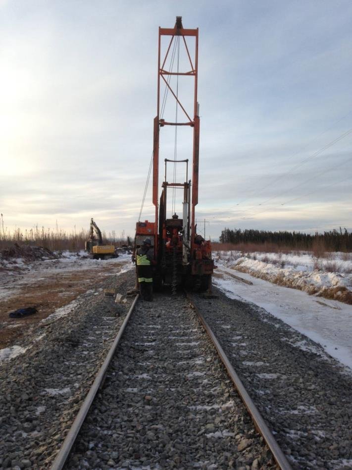
After Geotechnology for Railroaders Program, Module 6.2; §05. Full reference under Supplemental Sources.
When piles are installed in a group, the group capacity may be less than the sum of individual pile capacities due to stress overlap. The group efficiency factor η is:
Reference graphics
η = 1 − θ · [(n−1)·m + (m−1)·n] / (90 · m · n)
Where:
AREMA MRE Chapter 7 requires center-to-center pile spacing of at least 2.5 pile diameters for driven piles and 3.0 diameters for drilled shafts. At S = 3D for driven piles (common for BNSF bridge pile groups), η ≈ 0.72–0.82.
For cohesive soils, the block failure mode must also be checked: the lesser of the group efficiency method and the block failure capacity controls.
Q_block = 2·D_g·(B_g + L_g)·su,avg + Nc·su,tip·B_g·L_g
Where:
Tension forces from wind uplift, seismic uplift, and locomotive-induced overturning at signal mast foundations must be checked. Net uplift capacity for a single pile:
Reference graphics
Q_ult,tension = Σ(f_s · As) + W_pile
Skin friction in tension is typically reduced to 75–80% of the compression value for driven piles (FHWA GEC No. 12). For CPKC and CN pile foundations in frost-susceptible soils, the adhesion of frozen soils to the pile during spring thaw can impose significant upward force ("frost heave uplift") that is distinct from structural uplift — a separate check is required per CN ES Chapter 5.
| Soil Type (USCS) | Consistency/Density | s_u or φ' | q_allow Shallow Fdn (tsf) | Railroad Application |
|---|---|---|---|---|
| CH (Fat Clay) | Very soft | s_u = 250–500 psf | 0.25–0.50 | Avoid; use piles — CSXT coastal GA |
| CL (Lean Clay) | Soft | s_u = 500–1,000 psf | 0.5–1.0 | Siding footings minimum 3 ft embed. |
| CL | Stiff | s_u = 1,000–2,000 psf | 1.0–2.0 | Bridge abutment footings — NSR |
| CL/ML | Very stiff | s_u = 2,000–4,000 psf | 2.0–4.0 | Grade crossing slabs — G&W |
| SM (Silty Sand) | Loose | φ' = 28–32° | 1.0–1.5 | Use piles for bridge loads — BNSF |
| SP (Poorly Graded Sand) | Medium dense | φ' = 32–36° | 1.5–2.5 | Signal foundations — UPRR |
| SW/GW | Dense | φ' = 36–40° | 2.5–4.5 | Intermodal crane footings — UPRR |
| GW (Well-graded Gravel) | Very dense | φ' = 40–45° | 4.5–7.0 | Mainline bridge piers — CPKC |
| CL over bedrock | Stiff clay cap | Mixed | 1.5–3.0 w/ piles to rock | NSR Appalachians |
| Limestone/Sandstone | Competent rock | RQD > 50% | 10–50+ | BNSF/UPRR bridge piers |
| Client | Preferred Pile Type | Minimum FS (w/test) | Minimum FS (no test) | Wave Equation Required | Load Test Required |
|---|---|---|---|---|---|
| CSXT | Driven concrete/pipe | 2.5 | 3.0 | Yes (WEAP) | Every bridge replacement |
| NSR | CIDH drilled shaft | 2.5 | 3.0 | N/A (drilled) | At 5% of shafts |
| G&W | HP steel piles | 2.5 | 3.0 | WEAP preferred | ≥1 per project |
| UPRR | HP/pipe driven | 2.5 | 3.5 | Yes (WEAP) | CAPWAP all piles |
| BNSF | Driven pipe/HP | 2.5 | 3.5 | Yes (WEAP) | CAPWAP ≥5% |
| CPKC | Driven pipe | 2.5 | 3.0 | Yes (WEAP) | ≥1 per bridge |
| Amtrak | Micropiles/CIDH | 2.0 | 2.5 | N/A | At every major rehab |
| CN | Driven pipe | 2.5 | 3.0 | WEAP required | ≥1 per structure |
| FRA (all classes) | Per AREMA Ch.7 | 2.5 min | 3.0 min | As applicable | Per client |
Reference graphics
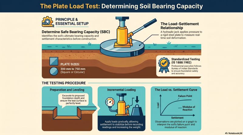
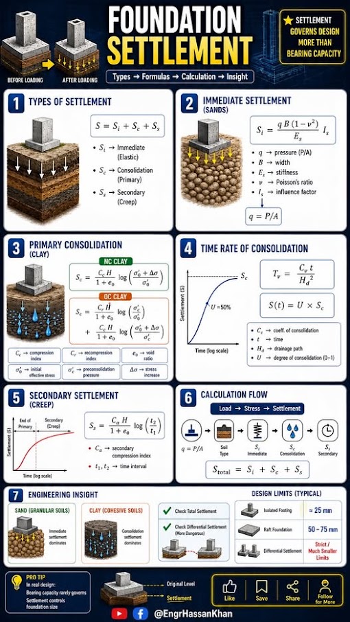
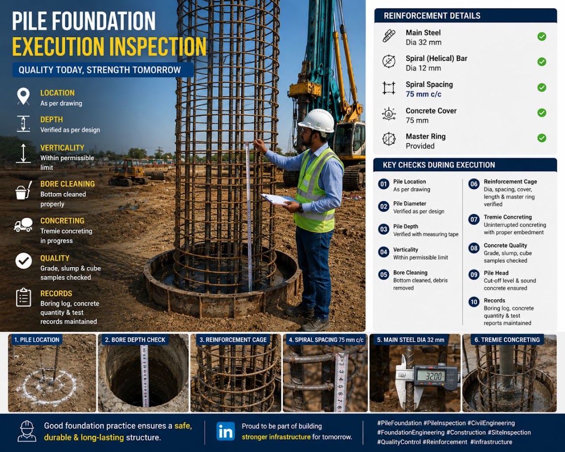
Project context: Norfolk Southern bridge replacement on the Pocahontas District, WV. Stiff residual CL clay, φ' = 24°, c = 600 psf, γ = 117 pcf. Proposed footing: 8 ft × 12 ft, D_f = 4 ft. Dead load = 280 kips, Cooper E-80 live load reaction = 165 kips, DLF = 1.30. Moment from earth pressure = 420 kip-ft about the short axis. NSR ESM requires FS ≥ 3.0 and eccentricity check per AREMA Chapter 8.
Step 1 — Design load and eccentricity
LL_factored = 165 kips × 1.30 = 214.5 kips
P_total = 280 + 214.5 = 494.5 kips
e_B = M / P = 420 kip-ft / 494.5 kips = 0.849 ft
B/6 = 8/6 = 1.33 ft → e_B = 0.849 ft < 1.33 ft ✓ (within middle third)
Step 2 — Effective dimensions
B' = 8 − 2(0.849) = 6.30 ft
L' = 12 ft (no eccentricity along length)
Step 3 — Bearing capacity factors at φ' = 24°
Interpolating from Table 11-1 between 20° and 25°:
Nq = 6.40 + 0.8(10.66 − 6.40) = 9.81
Nc = (9.81 − 1) / tan(24°) = 8.81 / 0.445 = 19.80
Nγ = 2(9.81 + 1) × tan(24°) = 2(10.81)(0.445) = 9.62
Step 4 — Correction factors
B'/L' = 6.30/12 = 0.525
Shape:
Fcs = 1 + (0.525)(9.81/19.80) = 1 + 0.260 = 1.260
Fqs = 1 + (0.525) tan(24°) = 1 + 0.234 = 1.234
Fγs = 1 − 0.4(0.525) = 1 − 0.210 = 0.790
Depth (Df/B' = 4/6.30 = 0.635 < 1):
Fcd = 1 + 0.4(0.635) = 1.254
Fqd = 1 + 2·tan(24°)·(1 − sin24°)²·(0.635)
= 1 + 2(0.445)(0.344)²(0.635)
= 1 + 2(0.445)(0.118)(0.635)
= 1 + 0.0668 = 1.067
Fγd = 1.0
Inclination: vertical load → Fci = Fqi = Fγi = 1.0
Step 5 — Overburden pressure at footing base
q = γ · Df = 117 × 4 = 468 psf
Step 6 — Ultimate bearing capacity
q_ult = c·Nc·Fcs·Fcd + q·Nq·Fqs·Fqd + 0.5·γ·B'·Nγ·Fγs·Fγd
= 600(19.80)(1.260)(1.254) + 468(9.81)(1.234)(1.067)
+ 0.5(117)(6.30)(9.62)(0.790)(1.0)
= 600(31.28) + 468(12.91) + 0.5(117)(6.30)(7.60)
= 18,768 + 6,042 + 2,801
= 27,611 psf
Step 7 — Allowable bearing pressure
q_allow = (q_ult − q) / FS + q
= (27,611 − 468) / 3.0 + 468
= 27,143 / 3.0 + 468
= 9,048 + 468
= 9,516 psf = 4.76 tsf
Step 8 — Applied pressure check
A_eff = B' × L' = 6.30 × 12 = 75.6 ft²
q_applied = P_total / A_eff = 494,500 lb / 75.6 ft² = 6,541 psf = 3.27 tsf
FS_actual = (q_ult − q) / (q_applied − q)
= (27,611 − 468) / (6,541 − 468)
= 27,143 / 6,073
= 4.47 ≥ 3.0 ✓
Conclusion: The 8 ft × 12 ft footing at 4 ft embedment is adequate with FS = 4.47 against bearing failure. NSR ESM requires submission of these calculations to the Bridge Engineering group for independent review. Settlement analysis for this footing (Chapter 12) must verify that total settlement < 1.0 in. and differential settlement < 0.75 in. across the span to maintain FRA Class 4 geometry tolerances.
Project context: BNSF Transcon main line, Kansas. Bridge pier replacement over seasonal stream. Soil profile: 0–15 ft fill (loose SM, φ' = 30°); 15–45 ft alluvial SP-SM (medium-dense, φ' = 35°, N₆₀ = 22 blows/ft); refusal on limestone at 45 ft. Use HP14×117 piles (area = 34.4 in², perimeter = 55.8 in = 4.65 ft). Pile tip at 43 ft (2 ft above rock). BNSF EI requires WEAP and CAPWAP.
Step 1 — Effective stress profile
Water table at 8 ft; γ_fill = 115 pcf; γ_SP-SM = 120 pcf; γ_w = 62.4 pcf:
At z = 15 ft (base of fill):
σ_v = 8(115) + 7(115 − 62.4) = 920 + 368 = 1,288 psf
σ'_v = 1,288 psf
At z = 43 ft (pile tip):
σ'_v = 1,288 + (43−15)(120 − 62.4) = 1,288 + 28(57.6) = 1,288 + 1,613 = 2,901 psf
Step 2 — β values by layer
For steel H-piles: δ = 0.8 × φ'
Fill (0–15 ft): φ' = 30°, K = 1.0 (driven pile densification), δ = 24°
β_fill = K·tan(δ) = 1.0 × tan(24°) = 0.445
SP-SM (15–43 ft): φ' = 35°, K = 1.2 (driven), δ = 28°
β_sand = 1.2 × tan(28°) = 1.2 × 0.532 = 0.638
Step 3 — Skin friction by layer
Pile perimeter = 4.65 ft
Fill layer (0–15 ft):
σ'_v,avg = (0 + 1,288) / 2 = 644 psf
f_s,fill = 0.445 × 644 = 286 psf
A_s,fill = 4.65 × 15 = 69.75 ft²
Q_s,fill = 286 × 69.75 = 19,948 lb = 19.9 kips
Sand layer (15–43 ft):
σ'_v,avg = (1,288 + 2,901) / 2 = 2,095 psf
f_s,sand = 0.638 × 2,095 = 1,337 psf
A_s,sand = 4.65 × 28 = 130.2 ft²
Q_s,sand = 1,337 × 130.2 = 174,017 lb = 174.0 kips
Step 4 — Tip resistance
Using Meyerhof Eq. 11-16 with N₆₀ = 22 in bearing sand, pile width B = 14 in = 1.167 ft, D_b = 28 ft (depth in SP-SM):
q_p = 0.4 × 22 × (28/1.167) = 0.4 × 22 × 24.0 = 211 tsf
but limited to 4 × N₆₀ = 4 × 22 = 88 tsf → governs
A_tip = 34.4 in² = 0.239 ft²
Q_p = 88 tsf × 2,000 lb/ton × 0.239 ft² = 42,064 lb = 42.1 kips
Step 5 — Total and allowable capacity
Q_ult = Q_s,fill + Q_s,sand + Q_p
= 19.9 + 174.0 + 42.1 = 236.0 kips
FS = 2.5 (with CAPWAP per BNSF EI)
Q_allow = 236.0 / 2.5 = 94.4 kips per pile
Step 6 — Design check
Cooper E-80 pier reaction for 80-ft simple spans (two-track bridge): ~800 kips total at pier.
Number of piles required = 800 / 94.4 = 8.47 → Use 9 piles (3×3 group)
Check group efficiency at 3D spacing (S = 3 × 14 in = 42 in = 3.5 ft):
m = n = 3; S = 3.5 ft; D = 1.167 ft
θ = arctan(1.167/3.5) = 18.4°
η = 1 − 18.4[(3−1)·3 + (3−1)·3] / (90 × 3 × 3)
= 1 − 18.4[12]/810
= 1 − 0.272 = 0.728
Q_group,allow = 9 × 94.4 × 0.728 = 618.8 kips < 800 kips
Group capacity is insufficient at 3D spacing. Increase to 4D spacing (S = 4.67 ft):
θ = arctan(1.167/4.67) = 14.0°
η = 1 − 14.0[12]/810 = 1 − 0.207 = 0.793
Q_group,allow = 9 × 94.4 × 0.793 = 673.7 kips < 800 kips (still low)
Design revision: Use 12-pile group (3×4) at 4D spacing:
θ = 14.0°; m = 3, n = 4
η = 1 − 14.0[(3−1)·4 + (4−1)·3] / (90·3·4)
= 1 − 14.0[8+9]/1080
= 1 − 14.0(17)/1080
= 1 − 0.220 = 0.780
Q_group = 12 × 94.4 × 0.780 = 883.5 kips > 800 kips ✓
Conclusion: A 12-pile group (3×4 arrangement) of HP14×117 piles at 4D center-to-center spacing provides Q_group,allow = 883.5 kips > 800 kips demand. BNSF EI requires WEAP analysis to establish refusal criteria and CAPWAP testing on a minimum of 5% of production piles. Pile tip elevations must be confirmed in the field; coordinate with BNSF Bridge Engineering per BNSF EI Section 3.4.
Project context: Union Pacific intermodal facility expansion, Dallas TX. Rubber-tired gantry (RTG) crane rail foundation. Design crane rail load = 180 kips per rail per axle, DLF = 1.20 (UPRR EIM). Proposed CIDH drilled shaft: 30 in. diameter, 35 ft deep. Soil: stiff CL, s_u = 1,800 psf (0–20 ft), very stiff CH, s_u = 3,200 psf (20–35 ft). UPRR EIM specifies α-method with FS = 2.5 (load test per project).
Step 1 — α values by layer
Layer 1 (0–20 ft): su = 1,800 psf, σ'v,avg ≈ 1,200 psf
ψ = 1,800/1,200 = 1.50 > 1.0 → α = 0.5(1.50^−0.25) = 0.5(0.904) = 0.452
Layer 2 (20–35 ft): su = 3,200 psf, σ'v,avg ≈ 2,400 psf
ψ = 3,200/2,400 = 1.33 > 1.0 → α = 0.5(1.33^−0.25) = 0.5(0.934) = 0.467
Step 2 — Skin friction by layer
Shaft perimeter = π × (30/12) = π × 2.5 = 7.854 ft
Layer 1 (0–20 ft):
f_s1 = 0.452 × 1,800 = 814 psf
As1 = 7.854 × 20 = 157.1 ft²
Qs1 = 814 × 157.1 = 127,879 lb = 127.9 kips
Layer 2 (20–35 ft):
f_s2 = 0.467 × 3,200 = 1,494 psf
As2 = 7.854 × 15 = 117.8 ft²
Qs2 = 1,494 × 117.8 = 175,993 lb = 176.0 kips
Step 3 — Tip resistance
Atip = π(2.5/2)² = π(1.25)² = 4.909 ft²
q_p = 9 × su,tip = 9 × 3,200 = 28,800 psf
Qp = 28,800 × 4.909 = 141,379 lb = 141.4 kips
Step 4 — Total and allowable capacity
Q_ult = 127.9 + 176.0 + 141.4 = 445.3 kips
Q_allow = 445.3 / 2.5 = 178.1 kips per shaft
Design load (factored) = 180 × 1.20 = 216 kips > 178.1 kips ✗
Step 5 — Revised design
Increase shaft diameter to 36 in. (perimeter = π × 3.0 = 9.425 ft; A_tip = π × 1.5² = 7.069 ft²):
Qs1 = 814 × (9.425 × 20) = 814 × 188.5 = 153,449 lb = 153.4 kips
Qs2 = 1,494 × (9.425 × 15) = 1,494 × 141.4 = 211,252 lb = 211.3 kips
Qp = 28,800 × 7.069 = 203,587 lb = 203.6 kips
Q_ult = 153.4 + 211.3 + 203.6 = 568.3 kips
Q_allow = 568.3 / 2.5 = 227.3 kips > 216 kips ✓ (FS = 2.63)
Conclusion: A 36 in. diameter CIDH shaft at 35 ft depth provides Q_allow = 227.3 kips with FS = 2.63 ≥ 2.5 per UPRR EIM. UPRR requires a static compressive load test (ASTM D 1143) prior to production shaft installation. Structural design of the crane rail mounting plate and anchor bolts is coordinated with UPRR Engineering and the crane manufacturer.
Reference graphics
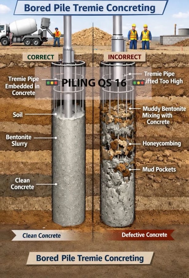
Weinhold’s chapter on special foundation works prices bored piles from a working-unit day rate. The day rate is the full cost of one rig with its crew, tooling and site containers for one workday, divided by realistic daily production.
The example rig is a cased Kelly rig, rated to 47 in diameter and 59 ft depth, with a 3-person crew on a 10-hour day. Its day rate includes:
Labor was about 28% of the day rate and the base machine about 40%.
The book’s shafts were 35 in diameter and 26–36 ft long, at a production rate of 164 ft per workday. Converted to US units, the cost per foot of shaft is made up of:
Reinforcing is a separate per-ton item. The other items are priced separately:
A flat 25% markup for overhead, risk and profit was considered acceptable, because bored piling is routine work for bidders.
The chapter lists the bid conditions that affect price:
It also notes that load tests on large projects can pay for themselves by allowing pile sizes to be optimized.
For railroad work: For bridge foundations and drilled-shaft retaining walls next to live track, the rig-day framework lets the engineer test how sensitive the cost is to geotechnical findings:
Production per workday should reflect the track windows actually available. Obstruction and standby items give the railroad unit prices for those risks instead of leaving them to claims.
Source: Jacob, D. and Müller, C. (Eds.) (2017). Estimating in Heavy Construction: Roads, Bridges, Tunnels, Foundations. Berlin: Ernst & Sohn, pp. 180–192. Summarized and paraphrased. Full reference under Supplemental Sources.
Values from these correlations are estimates, not test results. State the equation ID and source when one is used, confirm the soil or rock is within its range, and calibrate against site testing before design.
Checklist · Part VI · Geotechnical Analysis
Pre-Design
Shallow Foundation Design
Pile Foundation Design
Deliverables
Question 6.1 A 6 ft × 6 ft square footing for a G&W signal equipment foundation is embedded 3 ft in stiff lean clay (φ' = 0, s_u = 1,500 psf, γ = 115 pcf). No inclination or moment loading. Compute q_ult and q_allow using FS = 2.5 (G&W EB).
Answer:
At φ' = 0: N_c = 5.14, N_q = 1.00, N_γ = 0.0.
Shape factors (B/L = 1.0, square):
Fcs = 1 + (1.0)(1.00/5.14) = 1 + 0.195 = 1.195
Fqs = 1 + (1.0) tan(0°) = 1.0
Fγs = 1 − 0.4(1.0) = 0.60 (irrelevant; Nγ = 0)
Depth factors (D_f/B = 3/6 = 0.5 < 1):
Fcd = 1 + 0.4(0.5) = 1.20
Fqd = 1.0 (φ' = 0)
Overburden: q = 115 × 3 = 345 psf
q_ult = su·Nc·Fcs·Fcd + q·Nq·Fqs·Fqd
= 1,500(5.14)(1.195)(1.20) + 345(1.0)(1.0)(1.0)
= 1,500(7.36) + 345
= 11,040 + 345
= 11,385 psf
q_allow = (11,385 − 345)/2.5 + 345 = 11,040/2.5 + 345 = 4,416 + 345 = 4,761 psf = 2.38 tsf
Question 6.2 Explain the significance of the effective width B' in eccentric footing design and when AREMA Chapter 8 requires the middle-third check.
Answer: When a foundation carries a moment in addition to a vertical load, the resultant force acts at an eccentricity e = M/P from the footing centroid, shifting the pressure distribution. The effective width B' = B − 2e replaces B in all bearing capacity equations, reducing the available contact area and thus the capacity. AREMA MRE Chapter 8 requires that the resultant fall within the middle third of the footing (e ≤ B/6) under unfactored loading to prevent tension at the footing edge and ensure the soil remains in uniform compression. If e > B/6, the footing must be widened, the load must be recentered through structural geometry changes (battered piles, wider cap), or the embedment must be increased to bring the resultant within limits. This check applies to all bridge abutment footings and retaining wall base slabs subjected to earth pressure moments.
Question 6.3 Using the Meyerhof SPT method, estimate the allowable capacity of a 12 in. diameter closed-end pipe pile driven to 40 ft in medium-dense SP sand (N₆₀ = 18 blows/ft, uniform throughout). D_b = 30 ft in the bearing stratum. Use FS = 3.0 (no load test).
Answer:
Pile diameter B = 12 in = 1.0 ft; perimeter = π × 1.0 = 3.14 ft.
Skin friction (Eq. 11-15):
f_s = 0.02 × 18 = 0.36 tsf = 720 psf
As = 3.14 × 40 = 125.7 ft²
Qs = 720 × 125.7 = 90,504 lb = 45.3 tons
Tip resistance (Eq. 11-16):
q_p = 0.4 × 18 × (30/1.0) = 0.4 × 18 × 30 = 216 tsf
Limit: 4 × 18 = 72 tsf → governs
Atip = π(0.5)² = 0.785 ft²
Qp = 72 × 2,000 × 0.785 / 2,000 = 72 × 0.785 = 56.5 tons
Total capacity:
Q_ult = 45.3 + 56.5 = 101.8 tons = 203.6 kips
Q_allow = 101.8 / 3.0 = 33.9 tons = 67.9 kips (no load test, FS = 3.0)
This estimate would be refined after WEAP analysis and confirmed by CAPWAP or static load test for UPRR/BNSF projects.
Question 6.4 A 4×3 pile group (12 piles total) of 16 in. square concrete piles is installed at 4.0 ft center-to-center spacing (S/D = 3.0). Compute the Converse-Labarre group efficiency and compare to the sum of individual pile capacities if each pile has Q_allow = 120 kips.
Answer:
D = 16 in = 1.333 ft; S = 4.0 ft
θ = arctan(1.333/4.0) = arctan(0.333) = 18.4°
m = 4 columns; n = 3 rows
η = 1 − θ[(n−1)m + (m−1)n] / (90·m·n)
= 1 − 18.4[(3−1)4 + (4−1)3] / (90 × 4 × 3)
= 1 − 18.4[8 + 9] / 1,080
= 1 − 18.4(17) / 1,080
= 1 − 312.8 / 1,080
= 1 − 0.290 = 0.710
Q_group,allow = 12 × 120 × 0.710 = 1,022 kips
Sum of individuals = 12 × 120 = 1,440 kips
Group efficiency reduces available capacity by 29%.
This reduction must be accounted for in the foundation design; if the required group capacity is close to the sum of individuals, the piles must be spread further apart (S/D = 3.5–4.0) or additional piles added.
Question 6.5 Why does Amtrak prefer micropiles for underpinning existing NEC structures rather than driven piles or conventional drilled shafts? What geotechnical parameters govern the micropile design?
Answer: Amtrak preferences micropiles for NEC underpinning for three operational reasons: (1) Micropile installation uses rotary percussion drilling with small-diameter casings (4–10 in.), producing minimal vibration that could disturb track geometry or existing foundations — critical on the NEC where subgrade disturbance can violate FRA Class 7 geometry tolerances (cross-level ≤ 0.5 in.); (2) Drilling rigs are compact and can operate within Amtrak's narrow track-access windows of 4–6 hours; (3) Micropile loads are transferred to competent rock or dense soil at depth, bypassing the compressible fill and alluvial materials common along the NEC corridor.
Governing geotechnical parameters for micropile design are: (a) grout-to-ground unit bond stress (f_b) in the bonded zone, which ranges from 15–45 psi for sands and 5–25 psi for clays based on FHWA ADSC micropile design manual; (b) bonded zone length L_b selected to develop the required capacity; (c) structural capacity of the steel bar/casing core. Capacity: Q_ult = f_b × π × D_drill × L_b. Amtrak ES requires load testing per ASTM D 1143 on 5% of micropiles with a test load of 200% of the design load.
Values from these correlations are estimates, not test results. State the equation ID and source when one is used, confirm the soil or rock is within its range, and calibrate against site testing before design.
| Topic | Chapter |
|---|---|
| SPT N₆₀ and (N₁)₆₀ correction procedures | Chapter 6 |
| CPTu tip resistance and friction ratio for soil profiling | Chapter 7 |
| Soil classification for bearing capacity input (c, φ', γ) | Chapter 8 |
| Groundwater and effective stress; scour potential | Chapter 9 |
| Settlement analysis (companion to bearing capacity) | Chapter 12 |
| Slope stability of embankment around abutments | Chapter 13 |
| Seismic and liquefaction effects on foundation capacity | Chapter 14 |
| Ground improvement where bearing capacity is inadequate | Chapter 17 |
| Retaining wall foundation design | Chapter 16 |
| Track subgrade stress distribution below ballast | Chapter 2 |
| Pile driving monitoring and CAPWAP | Chapter 15 |
| Foundation analysis documentation in geotechnical reports | Appendix E |
| Consolidation and triaxial test data for c, φ', s_u input | Chapter 10 |
End of Chapter 11 — Foundation Engineering: Bearing Capacity
Primary source: USACE EM 1110-1-1804, Geotechnical Investigations (January 2001). Bearing capacity equations follow Vesić (1973) as presented in FHWA GEC No. 5, AASHTO LRFD Bridge Design Specifications, and AREMA MRE Chapter 8.
Authors: Daniel P. Colwell and Mario Ruel. This chapter was written and compiled by Daniel P. Colwell and Mario Ruel for Railway Ground Hazard Risk Management.
Technical content is drawn from the published sources below, and credit for that material belongs to their authors and publishers. Tables, equations and figures taken from a specific source are also cited where they appear.
File locations for these documents are listed under Supplemental Sources — LEVI Library.
Material in the green “Supplemental reference” boxes throughout this chapter was added from the following documents in the LEVI geotechnical library. Text is summarized or paraphrased; tables are reproduced with their original source noted; figures are reproduced from the cited document for internal reference use. Consult the original document before relying on a value for design. Blocks marked “After Selig & Waters (1994)” summarize item S7 for railroad clients; tables are condensed from the book and its figures are not reproduced. Blocks tagged “Project management” summarize methods, examples and figures from the project-management, estimating and construction-management books listed here, applied to railroad work; the closing “For railroad work” note in each block is added by the authors of this manual.